5 Functions of Excel/Sheets That Every Professional Should Know

I first used Microsoft Excel as a teenager, fumbling through receipts as I tried to organize numbers into a spreadsheet and later into QuickBooks. I was helping my dad’s friend prepare for his tax return, and I got a few bucks out of the deal. I’m not sure why he trusted a 16-year-old (with zero spreadsheet experience) to handle something like this. I couldn’t help but think, “He just gave me this job to be nice,” as I yelled at Clippy, the paper clip character, for not getting out of the way after it failed to help me as it claimed it would.

Related Content:

• Online Reputation Management
• Digital PR Services
• Content Marketing Agency
• Content Creation Services
• Custom Website Development Services

Now, many years after that, I look back and am grateful for getting that then-frustrating task. It was the foundation for a career that started in .XLSX, and I use this file type daily at Go Fish Digital. On our content marketing team, we often leverage data for our clients’ campaigns. This allows us to produce compelling material for journalists to use in their stories, and consequently earn backlinks and news coverage for our clients.

Even if you aren’t in a data-heavy field like marketing or SEO, a general understanding of spreadsheets has become essential for any working professional. Microsoft Excel and Google Sheets are the two major tools you’ll encounter and are structured very similarly. Below is a guide to five functions of either tool you can use to successfully manage data.

What Are The 5 Basic Excel Functions?

These are the 5 basic Excel functions that everyone should know:

1. The VLookup Function
2. The Concatenate Function
3. Text to Columns
4. Remove Duplicates
5. Pivot Tables

VLookup Excel Function

Example:

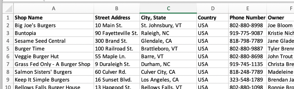
You have a spreadsheet of burger shops, and each individual one is listed out in column A, with their street address, city, state, owner name, annual sales, and other information in adjacent columns.

Among your long list of burger shops, there are only a handful you need information about. You could theoretically scroll through the spreadsheet or try to sort/filter the list, or you could use a Vlookup function to pull out the exact pieces of information you need. There are many use cases for this formula, and the more you become familiar with it, the more often you’ll find ways to use it to save yourself some time.

How To Set It Up:

• Create a new table in another tab if you don’t have one created already.

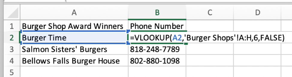
• In the first column, you’ll have the “lookup value,” which is the piece of information you’re telling the formula to look for in your main spreadsheet. This information will need to be in the left-most column of the table you’re telling the formula to look at, as it is in the first screenshot above.
• Then add the formula to the adjacent cell as follows:

=VLOOKUP(lookup_value,table_array,col_index_num,[range_lookup])

lookup_value: The cell where the formula can find the information that it needs to look up in your primary table. In this case, when putting the formula in cell B2, this value would be A2.

table_array: The table the formula should search and pull information from. Since my table of burger shops is on the tab named “Burger Shops” and I have data in columns up to column H, this value would be ‘Burger Shops’!A:H.

col_index_num: This is your way of telling the formula what information you want it to bring back for you. In this example, I’m looking for the phone number, which is in column F in my main table. F is the 6th letter in the alphabet, and so this value in the formula will be 6.

[range_lookup]: This is a logical section of the formula, where the options are TRUE or FALSE. If you put TRUE, the formula will return a value based on the closest match to your lookup value, even if it’s not the exact one. If you put FALSE, then it’ll only return a value if it finds the exact lookup value you referenced. In most cases, and in this burger shop example, we’ll want to put FALSE

Final formula:

=VLOOKUP(A2,’Burger Shops’!A:H,3,FALSE)

Concatenate Formula

Example:

Continuing the burger shop example, let’s say you want to have the city and state in one column. Perhaps you want to analyze the data by city, but there are cities with the same name in different states so you need them combined. The concatenate function is an incredibly easy formula that you can use to combine the contents of different cells.

How To Set It Up:

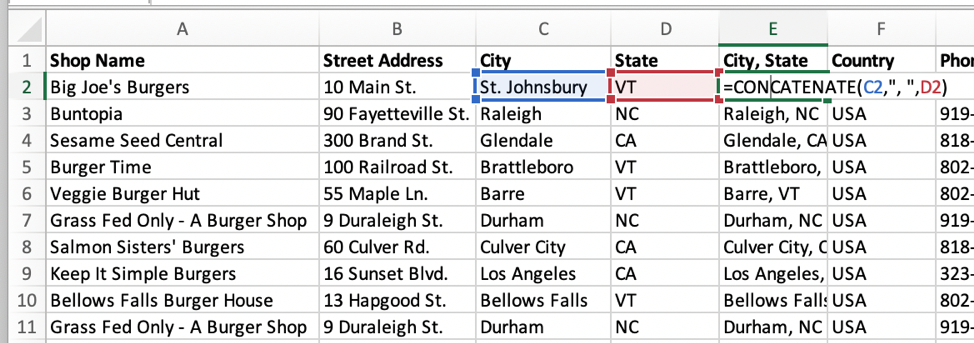
• First, you’ll need to add a new column to your table, which is where the new combined data will live

• Next, you’ll add the formula as follows:

=CONCATENATE(text1,text2,…)

You can type text and/or reference cells in this formula, which makes it very versatile. To add text, you’ll just type in what you want and add quotation marks around it. In this example, we’ll want to add a comma and space between the city and state.

Final formula:

=CONCATENATE(C2,”, “,D2)

Text to Columns Excel Function

Example:

Let’s say you have the opposite problem as the previous example – you have city and state combined for each burger shop, but you’d like them in separate columns. The “Text to Columns” function is a simple way of breaking data into multiple columns based on certain criteria. It can separate text based on a space or a certain delimiter, such as a dash or comma.

How To Set It Up:

• Add a column to the right of the column you’re separating (or multiple columns if you’re separating the data into more than two sections) like in the screenshot below

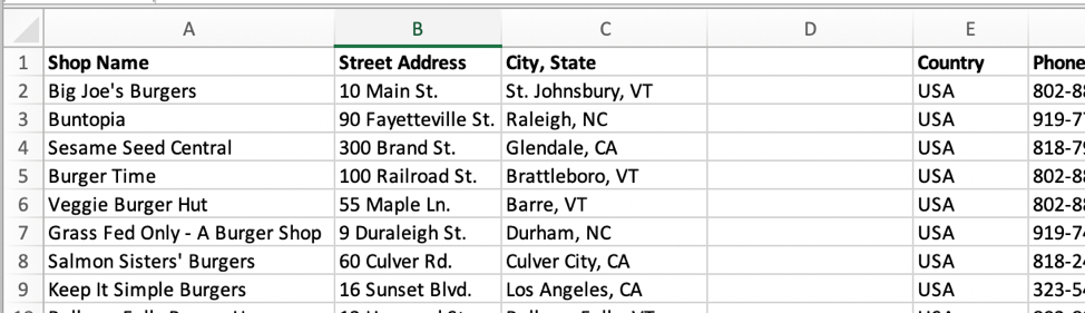
• Highlight the entire column with your text to be separated (in this case it’s column C)
• Click the “Data” tab in the toolbar
• Click “Text to Columns”
• Confirm that “Delimited” is selected
• Click “Next”
• Then select the delimiter that applies

In the burger shop example, the delimiter that applies is a comma, so I’d make sure that only the “Comma” checkbox is selected. At this point with a simple Text to Columns operation, you can click “Finish” and you will find your data split. You may have to update the column titles.

Remove Duplicates

Example:

In this burger shop spreadsheet, it may be the case that the same burger shop is listed multiple times. If you’re planning to analyze this data in a pivot table in the form of counts or averages, then you definitely don’t want any duplicate values in the dataset.

In this example, each burger shop has a unique name so any two rows with the same shop name indicate a duplicate that should be removed. If you’re using a spreadsheet where there are multiple items with the same title in a certain cell, though they are different based on their street address or city or otherwise, then you can use a simple Concatenate formula (see above) to create a unique “name” for each item in your table, then remove duplicates based on that.

How To Set It Up:

• First, you’ll highlight all of the columns in your table by clicking the first column (column A) and dragging your mouse over to the last relevant one.

• Next, you’ll click “Data” from the toolbar then “Remove Duplicates.” A window will appear and you’ll uncheck every column except for the one with the values that should be unique. In this example, it’s column A because it has the burger shop names.

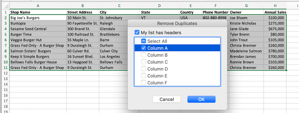
• Lastly, click “OK” and Excel will notify you of how many duplicates, if any, were removed. That means that Excel deleted all data in the row where a duplicate was found.

Pivot Tables

Example:

Let’s say you want to see how annual sales compare across states. Pivot tables allow you to take a dataset and summarize it in a variety of ways. It’s one of the most useful functions of Excel or Sheets.

How To Set It Up:

• Navigate to your table of data and click anywhere within it
  • There’s no need to manually highlight all of your relevant cells unless you aim to exclude certain rows or columns from your pivot table – the pivot table function will automatically pull in all data within a complete table that does have any breaks
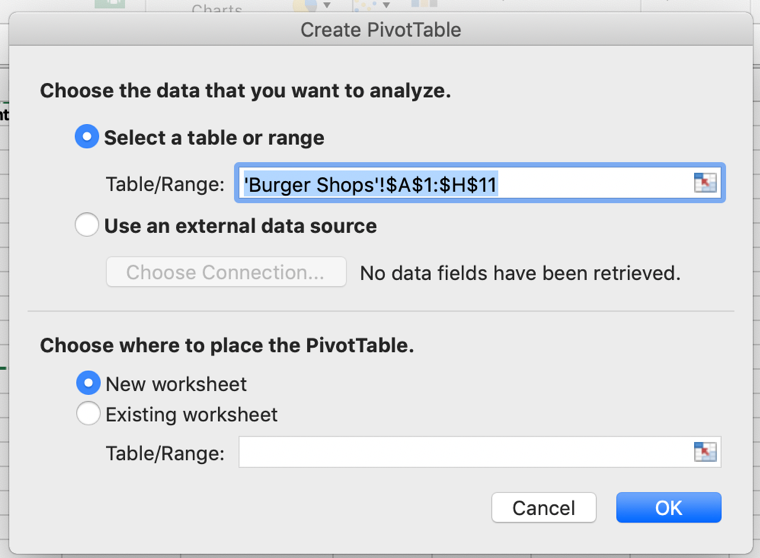
• Under the “Insert” section in Excel or “Data” section in Sheets, click “PivotTable”
• In Excel, a window will appear, and you’ll click “OK.” You’ll now be able to set up your pivot table to summarize your data how you’d like

• To get the average annual sales by state example, drag “State” from the Field Name list to the section titled “Rows”
• Drag “Annual Sales” to the section titled  “Values”
• For this example, we want to see the average of these values, not the sum. To change that, click the “i” icon beside “SUM of Annual Sales” in the “Values” sections, then select “Average” from the list that appears

• You’ll then have the average annual sales by state

Other Use Cases:

There are endless ways to use pivot tables – it’ll just depend on the dataset you’re analyzing. In a spreadsheet of houses for sale, you could find the count of houses for sale by city or state. In a table of revenue by month for the past four years, you could find the average amount of revenue by month or quarter of the year. You can also set up more complex pivot tables that include calculated fields.

Closing Thoughts On Excel Functions

Admittedly, the first time you use one of these functions, it might be a frustrating experience of trying to make it work. I’d urge you to stick with it if this happens. A solid grasp of these essential functions is valuable in any industry that requires that you use data — which is nearly all of them. The more you practice, the easier and quicker you’ll get at using spreadsheets, and the more time you can save yourself when putting together analyses in the future.